Nov 08 2024 • 5 min read

Deep Dive: Hessians

Recently, I was taught the second derivative test for multivariable functions $f(x, y)$, which goes something like this:

Let $(x, y)$ be a critical point of $f$, and define $D$ to be $f_{xx}(x, y) f_{yy}(x, y) - f_{xy}(x, y)^2$. Then we have:

$$(x, y) = \begin{cases} \text{local max/min} & D > 0 \\ \text{saddle} & D < 0 \\ \end{cases}$$

If $D = 0$, the test is inconclusive.

No proof was given, so I decided to go and try to find my own intuition and ended up discovering some fascinating things along the way.

I. MOTIVATION

The first question we should ask ourselves is: what visual properties do a function’s extrema and saddle points have in 3D?

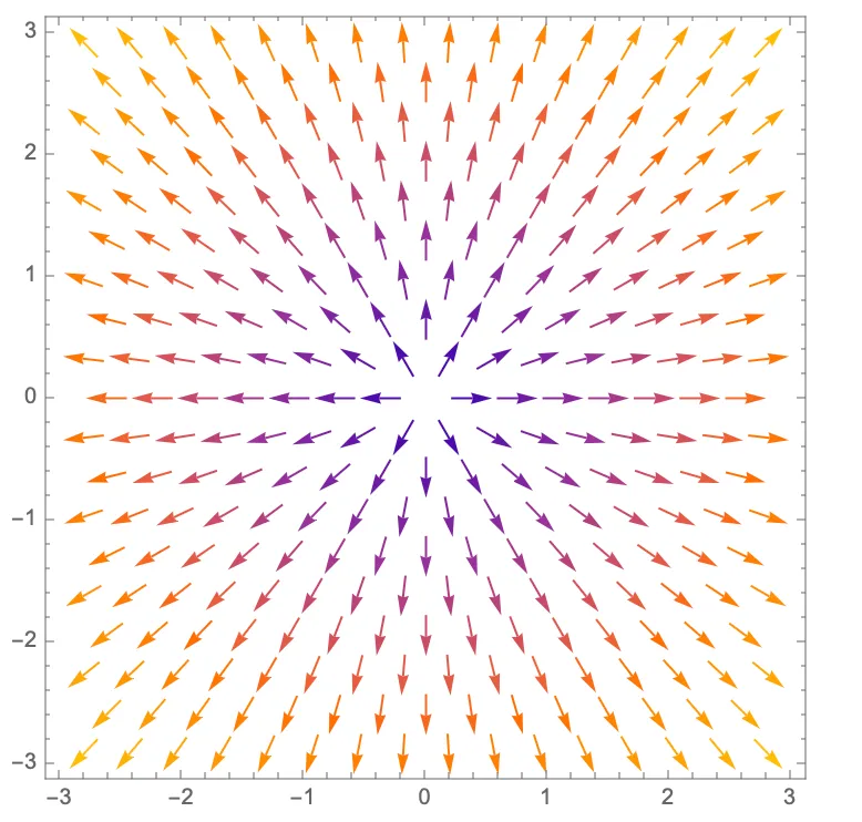
There are several ways to answer this question, but I will begin by considering the function’s gradient field. For instance, here’s the gradient field for $z = x^2 + y^2$:

We can clearly see that all the gradients point away from the local minimum; for a local maximum, it would be the opposite.

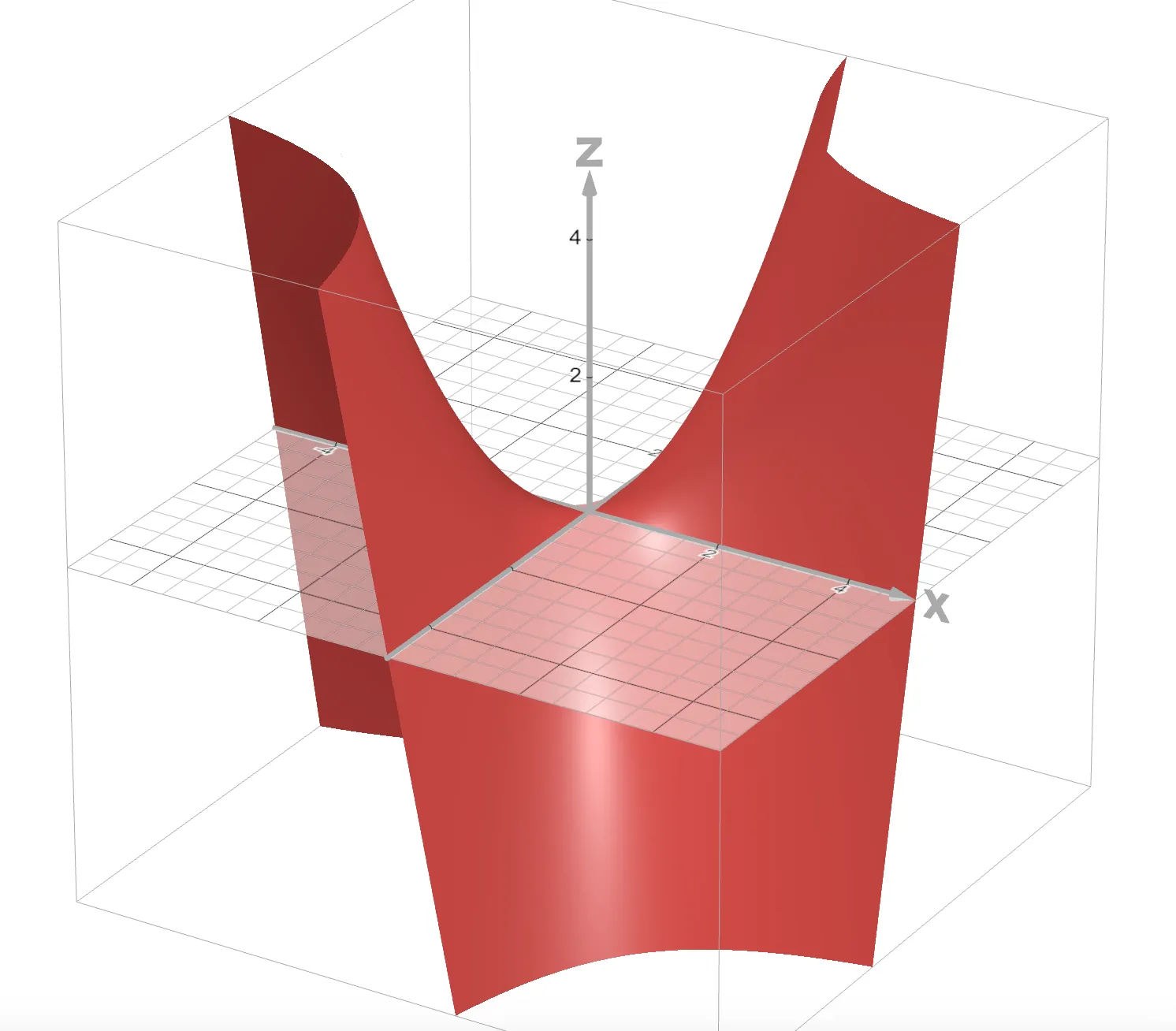
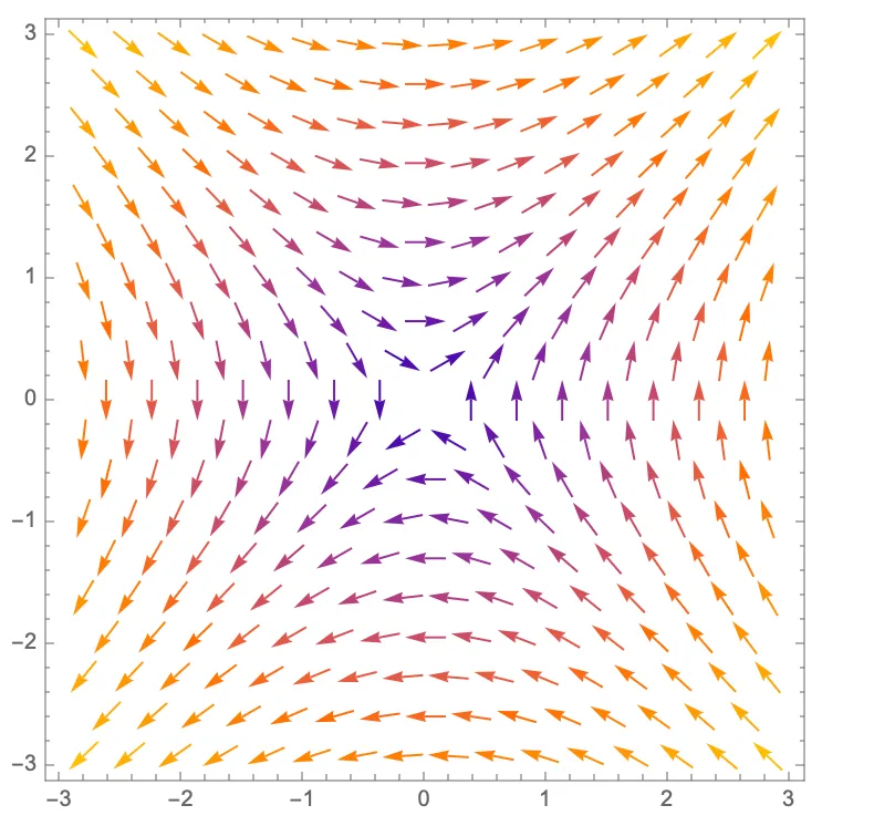
On the other hand, here’s the plot and gradient field of $z = xy$, a clear saddle shape:

Plot	Gradient field

Here, we see some vectors pointing toward the critical point, while some point away. This makes sense as a saddle point is, by definition, a local max along some paths and a local min along others.

These observations thus motivate a method to quickly check whether the gradients in the neighborhood of $(x, y)$ point away from, toward, or in both directions from $(x, y)$, which brings us to…

II. HESSIANS

A Hessian in 2 dimensions is defined like so:

$$H_f = \begin{bmatrix} f_{xx} & f_{xy}\\ f_{yx} & f_{yy} \end{bmatrix}$$

Immediately, we recognize $D$ as the determinant of this matrix. As we will soon find, this is no coincidence.

Note: for all following explanations, assume WLOG that the critical point $(x, y)$ in question is $(0, 0)$.

But first, let’s think about what this matrix is telling us. Let’s multiply it by the vector $\langle dx, dy \rangle$:

$$\begin{bmatrix} f_{xx} & f_{xy}\\ f_{yx} & f_{yy} \end{bmatrix} \begin{bmatrix} dx \\ dy \end{bmatrix} = \begin{bmatrix} d\frac{df}{dx} \\ d\frac{df}{dy} \end{bmatrix} = d(\nabla f)$$

In words, this multiplication tells us how much a move by $\langle dx, dy \rangle$ will change the function’s gradient. Moreover, since $\nabla f(0, 0) = \vec{0}$,

$$\nabla f(dx, dy) = \nabla f(x, y) + d(\nabla f) = 0 + d(\nabla f) = H_f\begin{bmatrix} dx \\ dy \end{bmatrix}$$

Thus, $H_f\begin{bmatrix} dx \\ dy \end{bmatrix}$ is simply a linear approximation of the gradient at $(dx, dy)$.

At this point, we should formalize what it means for the field to point away from or toward the origin. If for all $\langle dx, dy \rangle$,

$$\begin{bmatrix} dx & dy \\ \end{bmatrix} H_f\begin{bmatrix} dx \\ dy \end{bmatrix} > 0$$

then all the gradients point away from the origin, and thus $(0, 0)$ is a local minimum (note that the left term is just the dot product between $\langle dx, dy \rangle$ and its approximated gradient). Take a moment to reason out the intuition behind this definition if you haven’t already.

Similarly, if these dot products are all less than 0, $(0, 0)$ is a local max; if some are greater than 0 and others are less than 0, we have a saddle point; and otherwise, the test is inconclusive.

Those well-versed in linear algebra might already see where this is going…

III. DEFINITE MATRICES

This Wikipedia article, in all its length, somehow manages to glance over key intutions, which I hope to cover here.

First, recall the Hessian must be a symmetric matrix, since $f_{xy} = f_{yx}$. An important property of all symmetric matrices is that they all correspond to a diagonal transform (i.e. a dilation, potentially non-uniform) on a rotated set of perpendicular axes.

The axes are shown here in red, and we can clearly see the dilation stretches along one of the axes and shrinks along the other.

As long as neither axis is dilated by a negative factor (i.e. is subject to a reflection), we can see intuitively that the resultant vector field will be pointing away from the origin. On the other hand, if both are dilated by negative factors, all the vectors will be pointing toward the origin. And if one stretch factor is negative and the other positive, we will have a mix of vectors pointing in both directions—this corresponds to the saddle case.

Now we see where the determinant comes in: if we think of the determinant of a matrix transform as the amount it scales area by, we can see that the determinant of our transform with stretch factors $a$ and $b$ should just be $ab$. If $a$ and $b$ are both positive or both negative, corresponding to the local minimum and local maximum cases, respectively, then the determinant will be positive. Otherwise, the determinant must either be less than 0, which corresponds to the saddle case, or 0, in which case the test is inconclusive.

IV. FURTHER READING

Hopefully, you’ve gained a better intuition for both Hessians and the second derivative test for multivariable functions. If you’re curious, here are some more concepts to explore:

• A symmetric matrix has perpendicular eigenvectors. N.B: you actually already saw this!
• The determinant of any matrix is the product of its eigenvalues.
• What does a matrix transpose mean visually?